- In the smaller models less electromagnetic generator power is required to produce measurable temperature rises. in full-size models excessive amounts of power are often required to produce measurable temperature rises, especially enough rise to measure heating patterns accurately in the presence of thermal diffusion.
- Use of several scaled models permits measurements at more frequencies. Since most lectromagnetic generators with sufficient power are narrow-band, measurements in full-size models can usually be made only over a very narrow frequency band
- Scaled models are smaller, easier to handle, and less expensive than full-size models.
Mathematical basis for Measurements on Scaled Models--The derivation of relations between quantities in the full-size and scaled system is outlined here. Readers interested only in the results should skip to the next subsection.
Figure 7.4.
Schematic diagram illustrating the coordinate
system used in the scaling procedure. (a) Fullsize object
with coordinate system x, y, z; (b) scaled model with
coordinate system  .
.
Each point in à is obtained by reducing the coor-dinates of a point in A by the scale factor S. Therefore, the coordinate values are related by
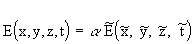 (Equation 7.13)
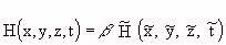 (Equation 7.14)
 (Equation 7.15)
where E is electric field; H is magnetic field; t is time; and
 are the corresponding scale
factors.
are the corresponding scale
factors.
where ![]() is the complex permeability and
is the complex permeability and  is the complex relative permittivity (see Sections
3.2.6, 3.3.3, and 4.1). The effective conductivity,
is the complex relative permittivity (see Sections
3.2.6, 3.3.3, and 4.1). The effective conductivity,  , is
related to e" by
, is
related to e" by
 (Equation 7.18)
Fields in the scaled model, on the other hand, must satisfy
where
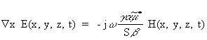 (Equation 7.21)
Note that
Equations 7.21 and 7.22 will be the same as 7.16 and 7.17, respectively, if
If material properties and scaling factors are selected so that Equations 7.25 and 7.26 are true, then measured quantities in the scaled model can be related to those in the full-size system, because Equations 7.19 and 7.20, which describe fields in the scaled system, are equivalent to Equations 7.16 and 7.17, respectively, which describe fields in the full-size system.
Second, it is most convenient to have both the
full-size and the scaled models surrounded dby air. Then
Equation 7.26 must be valid when both ![]() and
and ![]() represent air; that is
represent air; that is ![]() From Equation 7.26 for this condition,
From Equation 7.26 for this condition,
Equations 7.27 and 7.28 together require
 (Equation 7.29)
 (Equation 7.30)
 from boundary
conditions. This is equivalent to adjusting the intensity of
the electromagnetic sources in the two systems. The usual
practice is to set
from boundary
conditions. This is equivalent to adjusting the intensity of
the electromagnetic sources in the two systems. The usual
practice is to set
 (Equation 7.31)
which is equivalent to making the intensity of
the source fields in the two systems equal. This can be seen
from Equations 7.13 and 7.14, which are valid for all pairs
of coordinate points (x, y, z, t) and  . Let the
corresponding points be far enough away from the object so
that scattered fields are negligibly small and only source
fields are present. Then, corresponds to the
source fields in the two systems having equal intensities.
This assumes that the sources in the two systems are
correspondingly similar. Since scattered-field intensities
are proportional to source field intensities, the
interpretation that "setting is equal to
making the source intensities equal" is valid at all
points but easier to understand at points where the scattered
fields are negligible.
. Let the
corresponding points be far enough away from the object so
that scattered fields are negligibly small and only source
fields are present. Then, corresponds to the
source fields in the two systems having equal intensities.
This assumes that the sources in the two systems are
correspondingly similar. Since scattered-field intensities
are proportional to source field intensities, the
interpretation that "setting is equal to
making the source intensities equal" is valid at all
points but easier to understand at points where the scattered
fields are negligible.
 (Equation 7.32)
 The relationship with the
effective conductivity, ![]() , is usually used. From Equations
7.26, 7.30, and 7.31,
, is usually used. From Equations
7.26, 7.30, and 7.31,
Relating ![]() and
and ![]() to
to ![]() and
and ![]() (see
Equation 7.18),
(see
Equation 7.18),

Using Equation 7.23 gives
 (Equation 7.34)
and using Equation 7.30 gives
 (Equation 7.35)
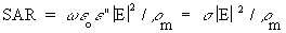
From Equations 7.32, 7.13, and 7.34, the general relationship for SAR is
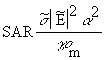 (Equation 7.36)
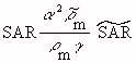 (Equation 7.37)
When both models are in air and the intensities
of the sources are equal (so Equations 7.30 and 7.31 apply) and for the usual case
when  , Equation
7.37 reduces to
From Equation 7.38, the scaled-model SAR is seen to be higher than that in the full-size model by scale factor S. This is often a significant advantage because it generally means that making measurements in a scaled model requires less generator power. This is particularly important when temperature measurements are made because it means that less power is required to get a measurable temperature rise in a scaled model than in a full-size model.
Another quantity that sometimes is of interest is the Poynting vector. The scaling relationship is easily obtained from Equations 7.13 and 7.14:
Adjusting the conductivity of the model material is often
important in scaling techniques, as illustrated in Table
7.15. This can usually be done by varying the amount of NaCl
in the mixture. Fortunately the amount of NaCl can be varied
enough to adjust  without affecting
 ![]() drastically. Figure 7
.5 shows conductivity as a function of percentage of NaCl for
various percentages of the gelling agent TX-150 (see Section
7.2.5). Doubling the percentage of TX-150 has a relatively
small effect on the conductivity, which is largely controlled
by the percentage of NaCl. Figures 7.6 and 7.7 show the
conductivity values as a function of percentage of NaCl.
These graphs can be used to simulate muscle tissue in saline
form for a wide range of frequencies and scale factors.
drastically. Figure 7
.5 shows conductivity as a function of percentage of NaCl for
various percentages of the gelling agent TX-150 (see Section
7.2.5). Doubling the percentage of TX-150 has a relatively
small effect on the conductivity, which is largely controlled
by the percentage of NaCl. Figures 7.6 and 7.7 show the
conductivity values as a function of percentage of NaCl.
These graphs can be used to simulate muscle tissue in saline
form for a wide range of frequencies and scale factors.
Table 7.14.
General Scaling Relationships
Table 7.15.
Scaling Relationships For Typical Values Of Scaling Parameters
Figures 7.5 and 7.6
Electrical conductivity of phantom muscle as
a function of NaCl and TX-150 contents measured at 100 kHz
and 23°C.
Figure 7.6
Electrical conductivity of saline solution as
a function of the aqueous sodium chloride concentration.
Figure 7.7
Electrical conductivity of saline
solution as a function of the NaCl concentration at 25ºC.
Table 7.16 shows nine compositions that can be used to
simulate muscle material over a wide range of parameters. For
example, to get a conductivity of  = 4.6 S/m, Figure 7.5 shows that the NaCl concentration should be about 3.5% of
the total mixture. From Table 7.16, we see that mixture VIII
could be adjusted to accommodate the 0.4% difference needed
in NaCl concentration. The
= 4.6 S/m, Figure 7.5 shows that the NaCl concentration should be about 3.5% of
the total mixture. From Table 7.16, we see that mixture VIII
could be adjusted to accommodate the 0.4% difference needed
in NaCl concentration. The  ' for the mixtures in Table 7.16
are all about that of water. In many cases the " for
biological tissue is the dominant factor in determining the
SAR, especially at frequencies from 10 to 20 MHz, and the
value of ' is not critical to the measurements.
' for the mixtures in Table 7.16
are all about that of water. In many cases the " for
biological tissue is the dominant factor in determining the
SAR, especially at frequencies from 10 to 20 MHz, and the
value of ' is not critical to the measurements.
Table 7.16.
Compositions of the Nine Mixtures Used for Measuring Dielectric Properties
7.3. TABULATED SUMMARY OF PUBLISHED WORK IN EXPERIMENTAL DOSIMETRY
Table 7.17 contains a summary of published work in experimental dosimetry, including references.
Table 7.17
A Summary of Available Experimental Data on Fields and SAR Measurements in Biological Phantoms and Test Animals Irradiated by Electromagnetic Fields
Go to Chapter 8.
Return to Table of Contents.
Last modified: June 14, 1997© October 1986, USAF School of Aerospace Medicine, Aerospace Medical Division (AFSC), Brooks Air Force Base, TX 78235-5301
This is a Department of Defense computer system for authorized use only. DoD computer systems may be monitored for all lawful purposes, including to ensure that their use is authorized, for management of the system, to facilitate against unauthorized access, and to verify security procedures, survivability, and operational security. Using this system constitutes consent to monitoring. All information, including personal information, placed on or sent over this system may be obtained during monitoring. Unauthorized use could result in criminal prosecution.
POC: AFRL/HEDM, (210)536-6816, DSN 240-6816